

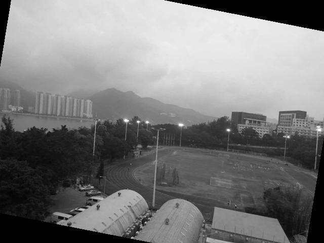
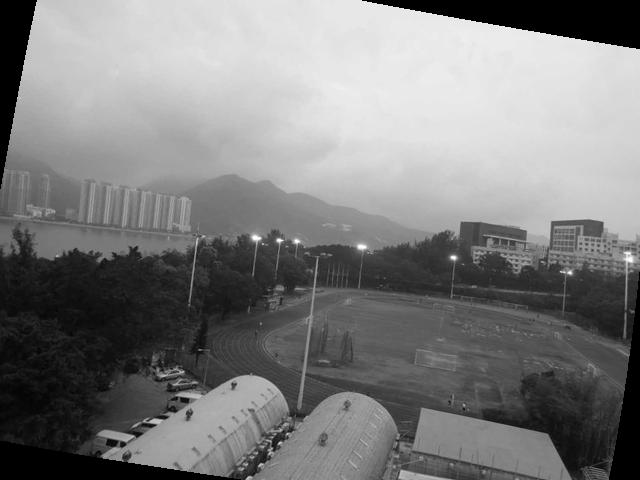
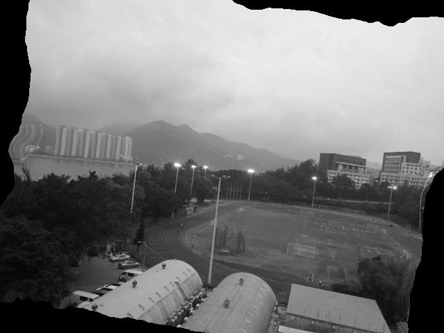
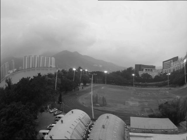
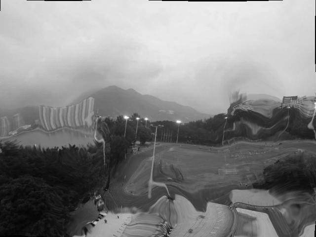

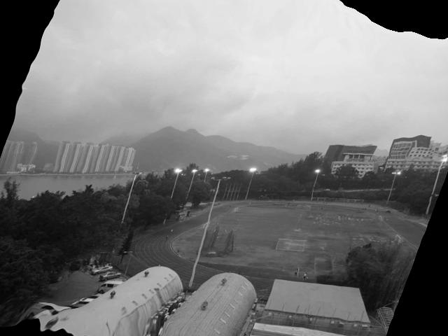
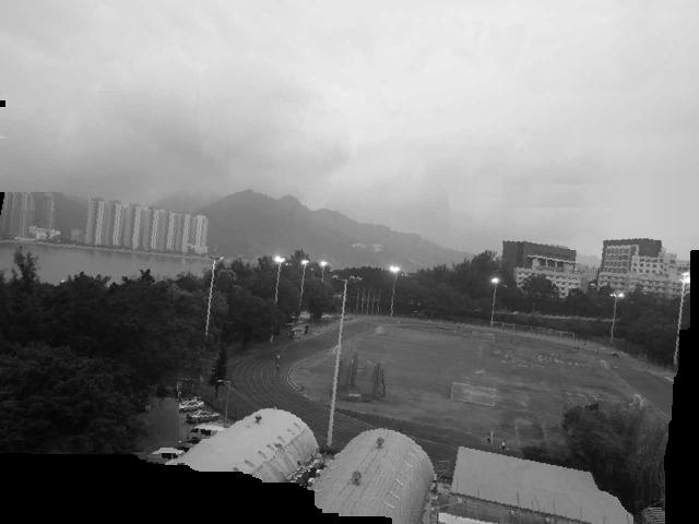
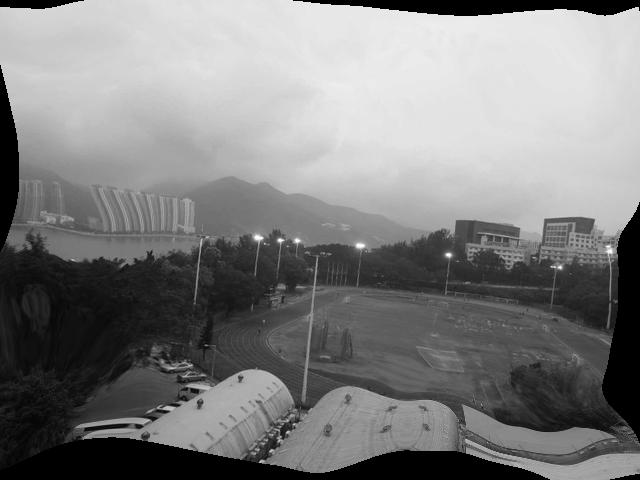
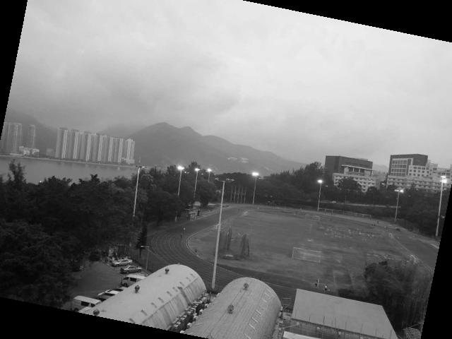
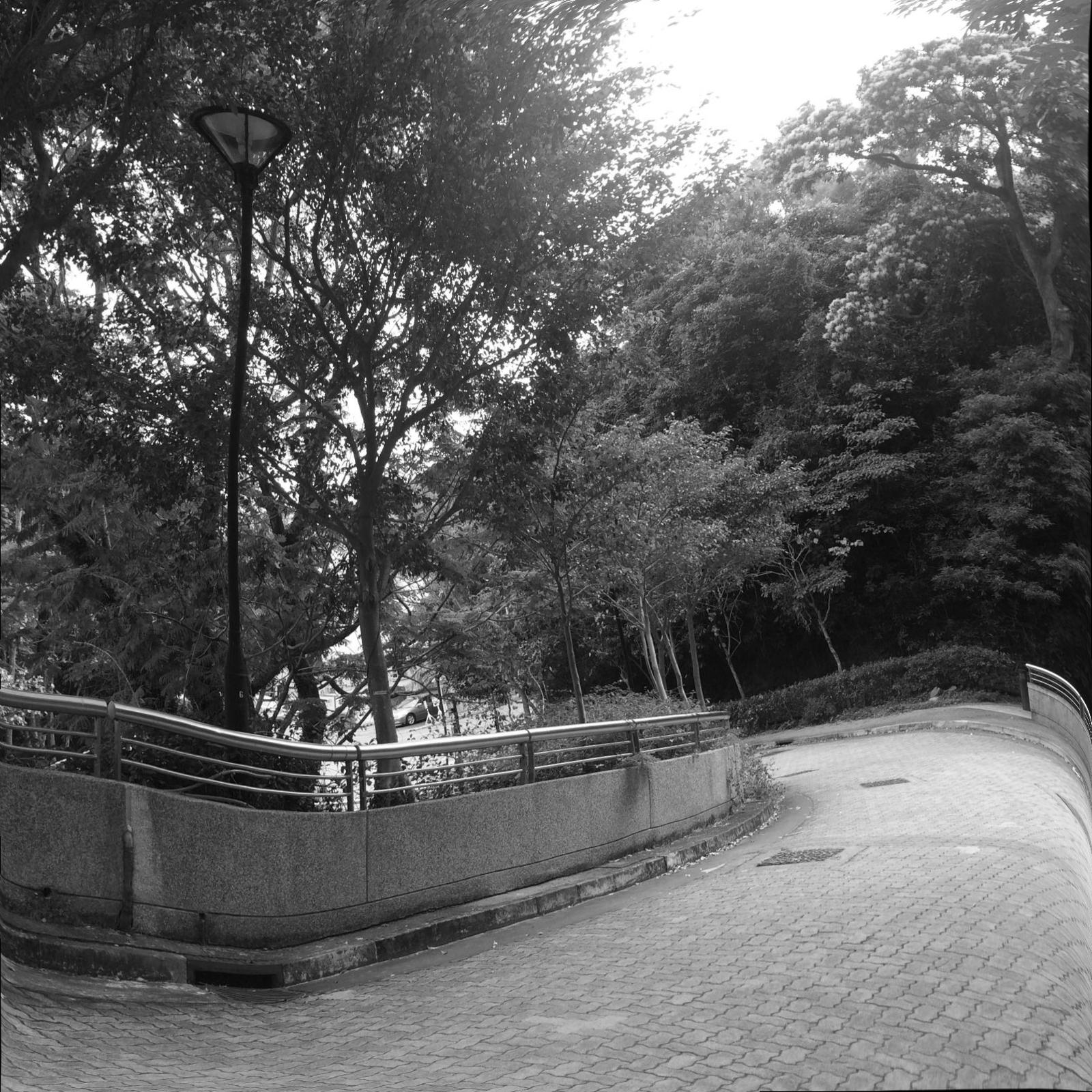
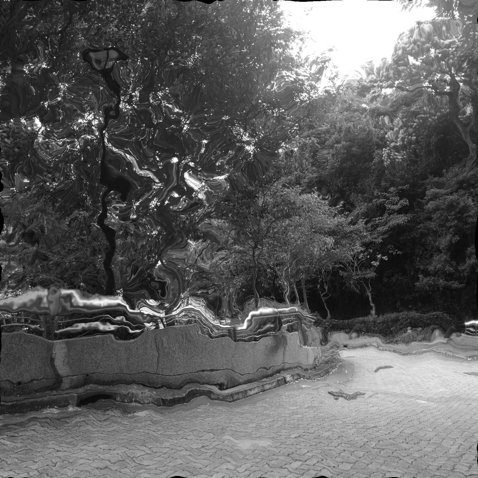
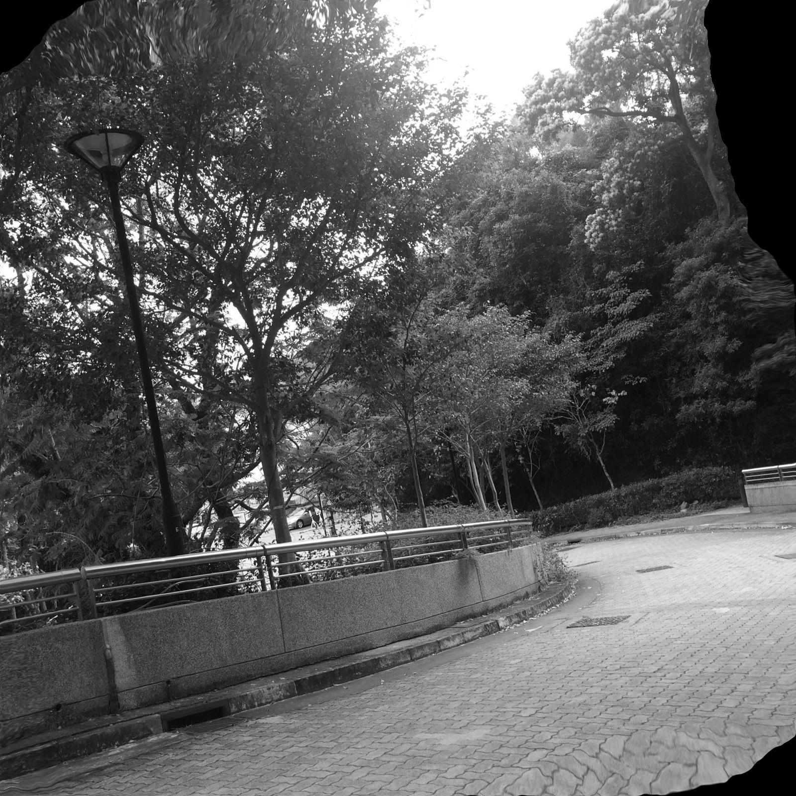
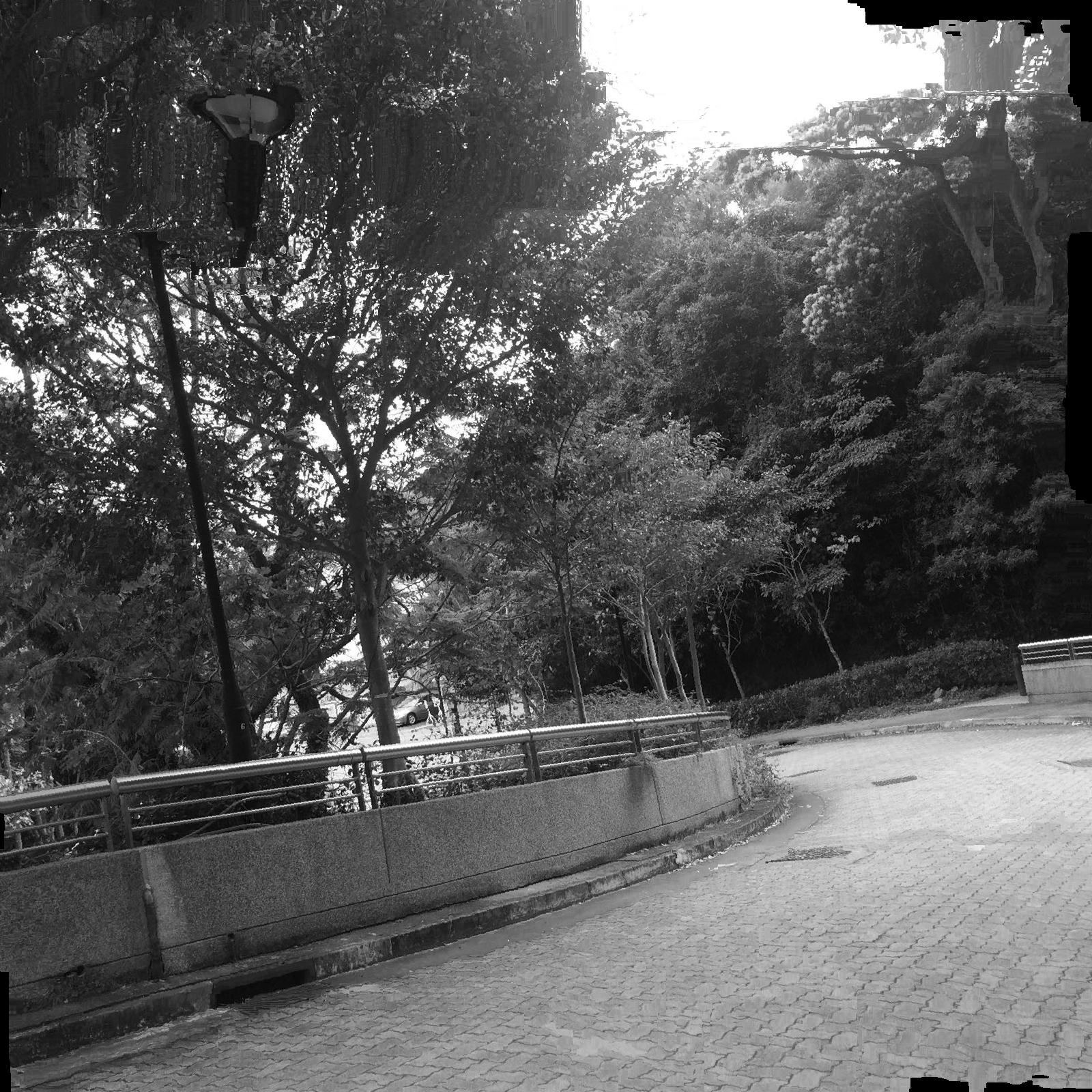
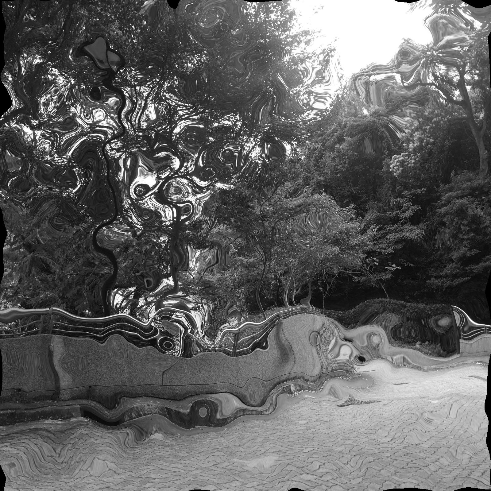
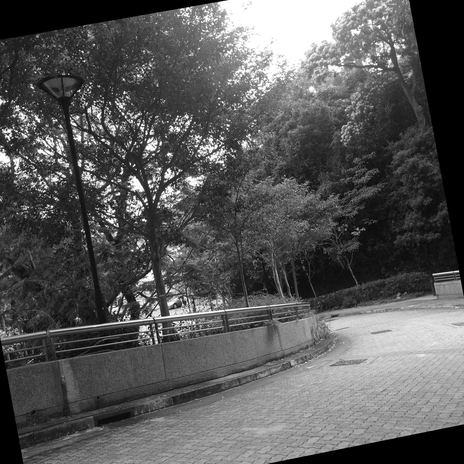
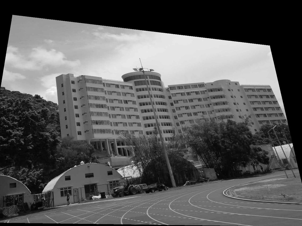
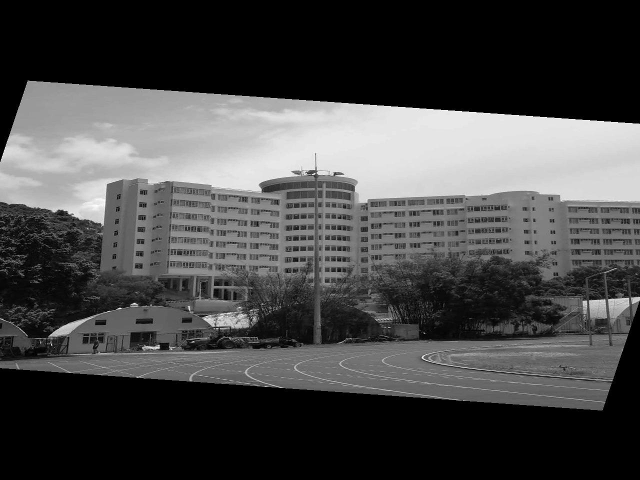
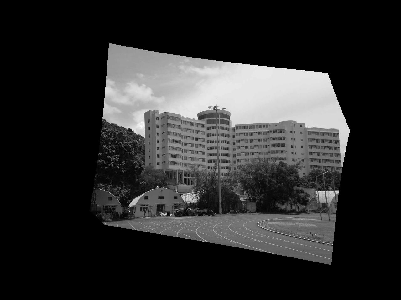
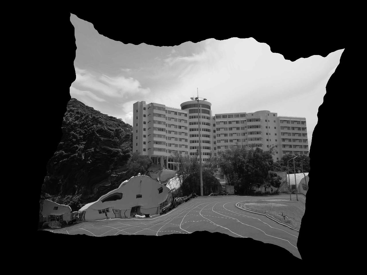
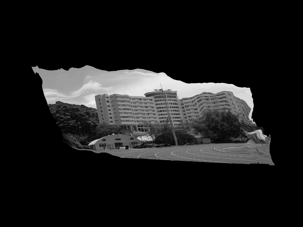
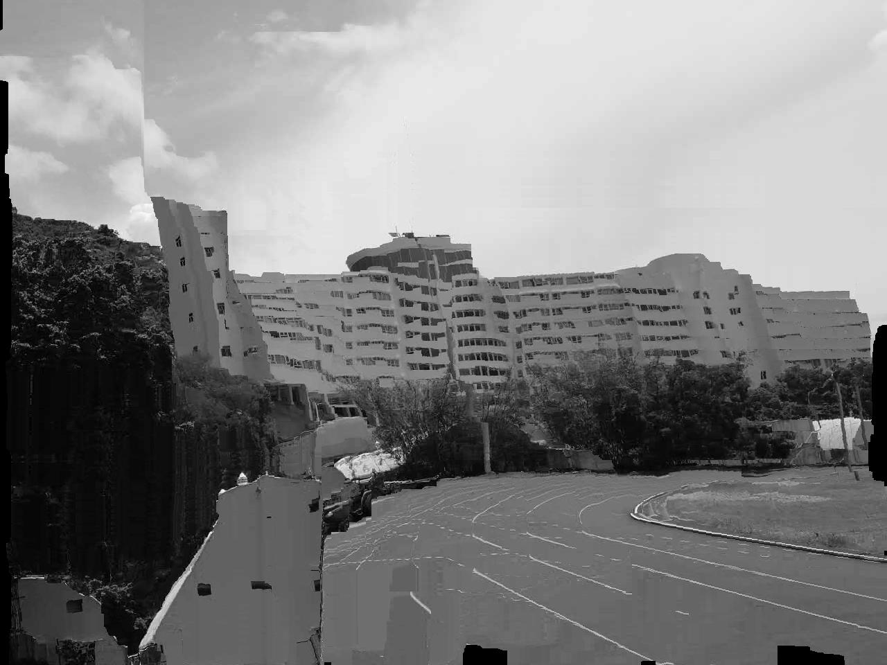
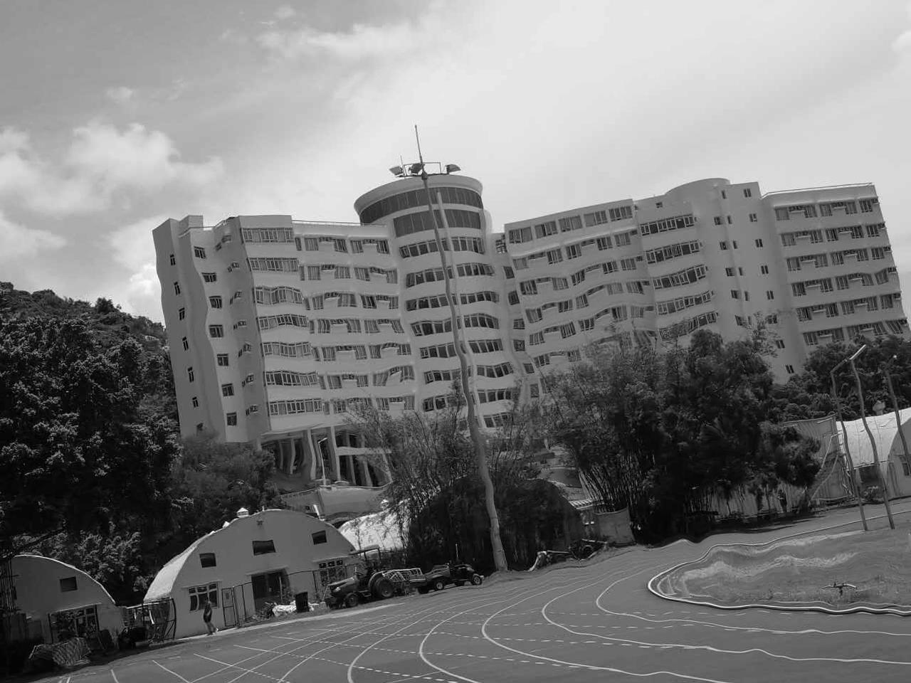
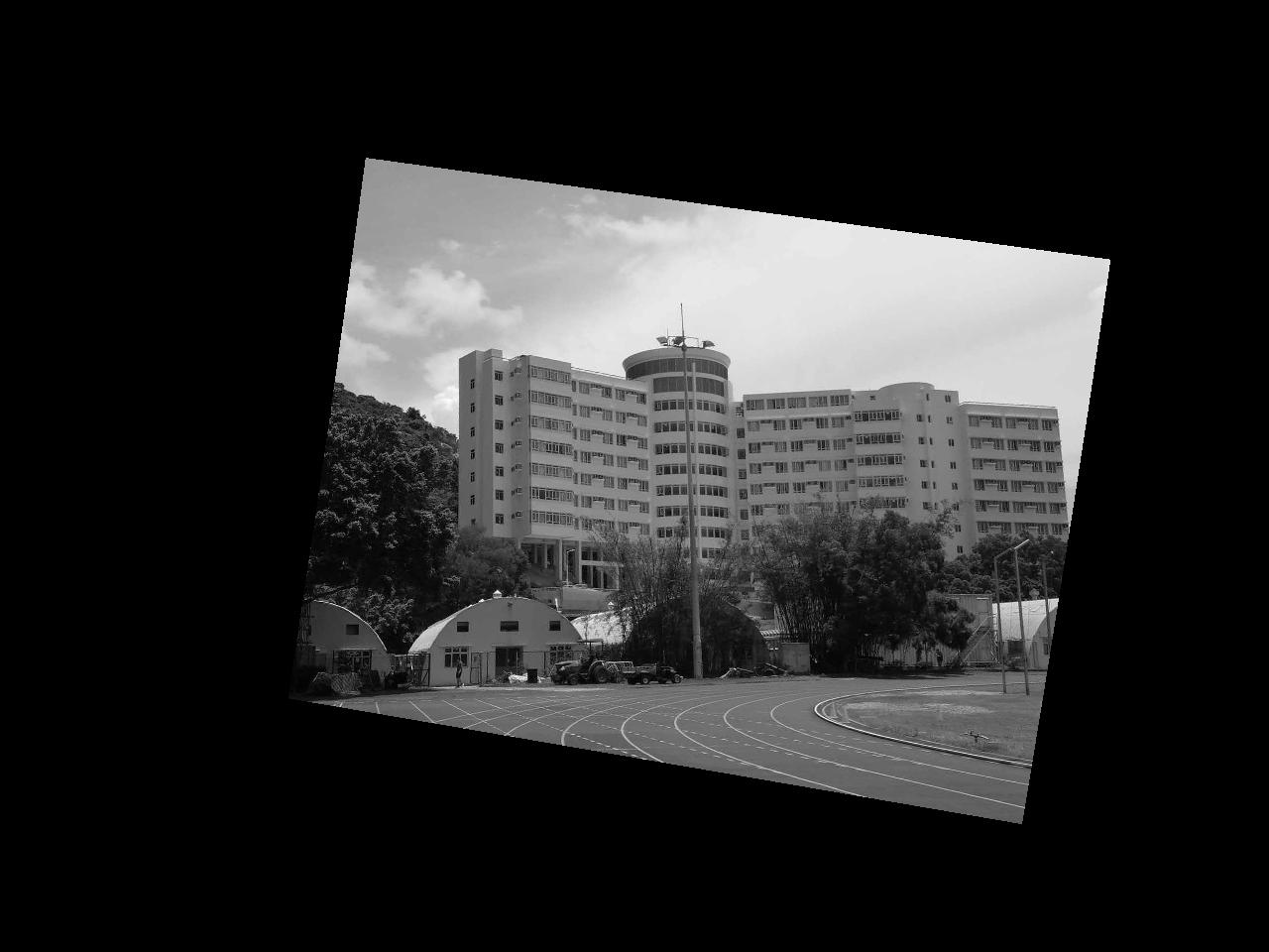
We show several comparing experimental results. We blend the target image (orange-toned) and the source image (blue-toned) to show the registration results. Perfect alignment is achieved when the blended image is tone-neutral (i.e., gray). The PSNR and computation time are shown below each image.
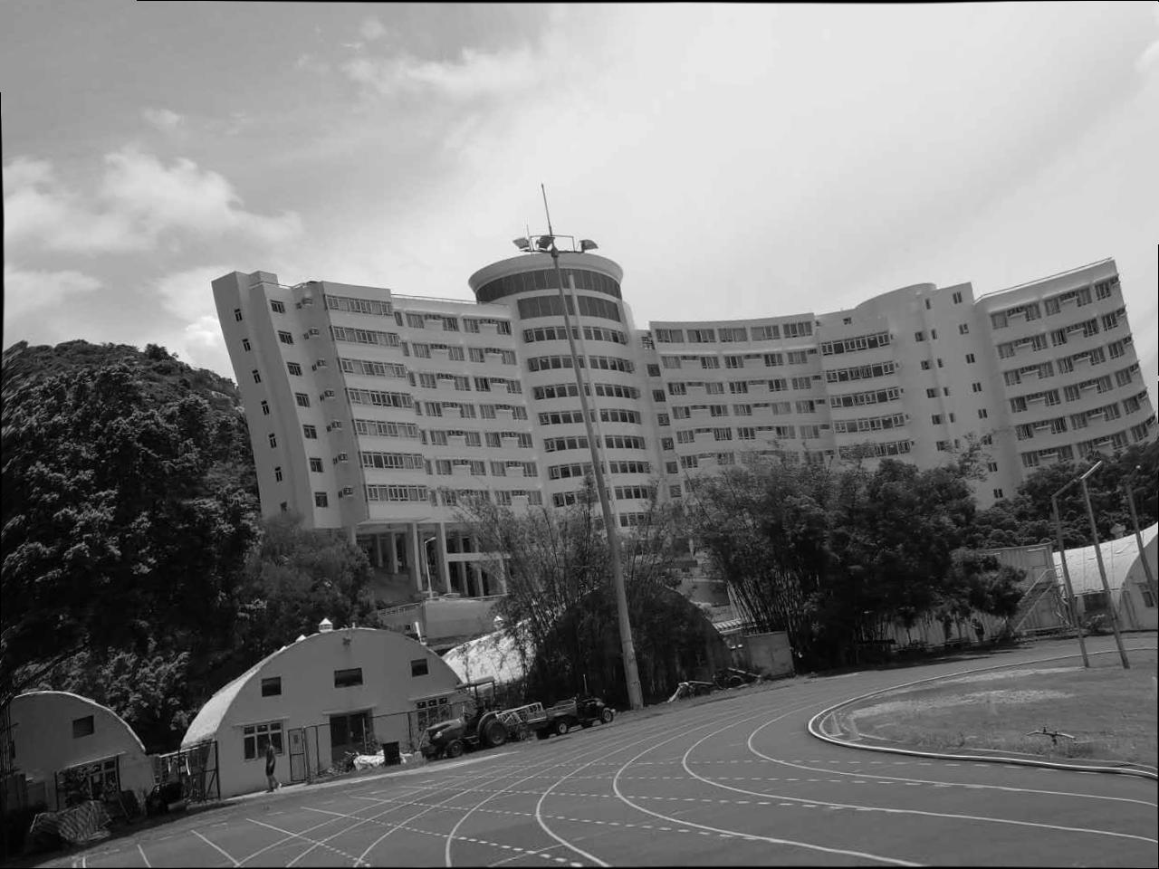
| Example 1. The size of the images are 480 × 640. | |||||
|
|
|
|
||
| (a) target & source | (b) ECC [1] | (c) NTG [2] | (d) LAFP [3] | ||
| 15.8 dB | 37.2 dB, 6.6s | 26.6 dB, 19.2s | 26.3 dB, 1574.4s | ||
|
|
|
|
||
| (e) LAP [4] | (f) Demons [5] | (g) MIRT [6] | (h) bUnwarpJ [7] | ||
| 35.3 dB, 9.4s | 18.9 dB, 152.8s | 17.4 dB, 46.3s | 23.1 dB, 10.4s | ||
|
|
|
|
||
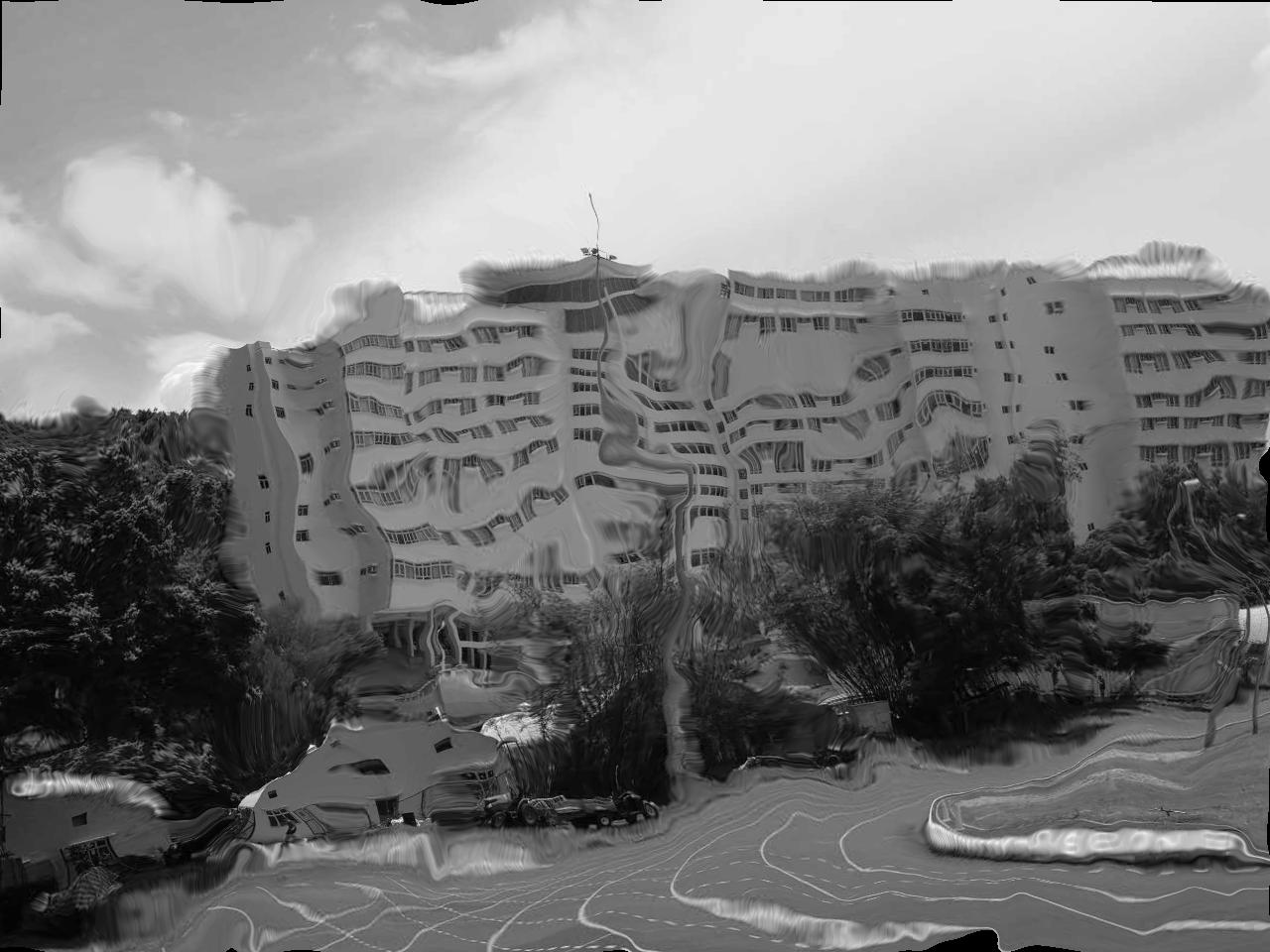
| (i) GIT [8] | (j) SIFT flow [9] | (k) Elastix [10] | (l) Ours | ||
| 19.1 dB, 419.9 | 28.9 dB, 37.2s | 21.9 dB, 229.4s | 38.2 dB, 4.4s | ||
| Example 2. The size of the images are 1600 × 1600. | |||||
 |
 |
 |
 |
||
| (a) target & source | (b) ECC [1] | (c) NTG [2] | (d) LAFP [3] | ||
| 12.3 dB | 13.0 dB, 61.3s | 18.3 dB, 46.6s | 18.2 dB, 1338.7s | ||
 |
 |
 |
 |
||
| (e) LAP [4] | (f) Demons [5] | (g) MIRT [6] | (h) bUnwarpJ [7] | ||
| 19.0 dB, 77.3s | 14.4 dB, 23.3s | 14.0 dB, 312.3s | 14.9 dB, 41.4s | ||
 |
 |
 |
 |
||
| (i) GIT [8] | (j) SIFT flow [9] | (k) Elastix [10] | (l) Ours | ||
| 22.0 dB, 3929.2 | 18.2 dB, 325.3s | 12.5 dB, 227.4s | 22.4 dB, 60.1s | ||
| Example 3. The size of the images are 960 × 1280. | |||||
 |
 |
 |
 |
||
| (a) target & source | (b) ECC [1] | (c) NTG [2] | (d) LAFP [3] | ||
| 12.2 dB | 13.0 dB, 29.9s | 10.0 dB, 25.0s | 21.5 dB, 1464.4s | ||
 |
 |
 |
 |
||
| (e) LAP [4] | (f) Demons [5] | (g) MIRT [6] | (h) bUnwarpJ [7] | ||
| 21.9 dB, 48.8s | 13.3 dB,11.2s | 12.6 dB, 85.6s | 14.5 dB, 25.3s | ||
 |
 |
 |
 |
||
| (i) GIT [8] | (j) SIFT flow [9] | (k) Elastix [10] | (l) Ours | ||
| 12.3 dB, 1766.9 | 15.5 dB, 152.8s | 12.2 dB, 109.5s | 27.4 dB, 38.6s | ||
| Example 4. The size of the images are 780 × 1040. | |||||
 |
 |
 |
 |
||
| (a) target & source | (b) ECC [1] | (c) NTG [2] | (d) LAFP [3] | ||
| 16.1 dB | 19.0 dB, 19.2s | 21.8 dB, 17.3s | 26.0 dB, 1744.1s | ||
 |
 |
 |
 |
||
| (e) LAP [4] | (f) Demons [5] | (g) MIRT [6] | (h) bUnwarpJ [7] | ||
| 25.4 dB, 12.6s | 19.3 dB, 53.9s | 17.6 dB, 73.3s | 21.7 dB, 16.7s | ||
 |
 |
 |
 |
||
| (i) GIT [8] | (j) SIFT flow [9] | (k) Elastix [10] | (l) Ours | ||
| 18.0 dB, 1766.5 | 30.8 dB, 100.2s | 19.2 dB, 226.5s | 37.1 dB, 11.9s | ||
| [1] | G. D. Evangelidis and E. Z. Psarakis, “Parametric image alignment using enhanced correlation coefficient maximization,” IEEE Transactions on Pattern Analysis and Machine Intelligence, vol. 30, pp. 1858–1865, 2008. |
| [2] | S.-J. Chen, H.-L. Shen, C. Li, and J. H. Xin, “Normalized total gradient: a new measure for multispectral image registration,” IEEE Transactions on Image Processing, vol. 27, no. 3, pp. 1297–1310, 2018. |
| [3] | Y. Matsushita, “Aligning images in the wild,” in IEEE Conference on Computer Vision and Pattern Recognition (CVPR), 2012, pp. 1–8. |
| [4] | C. Gilliam and T. Blu, “Local all-pass geometric deformations,” IEEE Transactions on Image Processing, vol. 27, no. 2, pp. 1010–1025, 2018. |
| [5] | H. Lombaert, L. Grady, and X. P. et al., “Diffeomorphic demons: Efficient non-parametric image registration,” NeuroImage, vol. 45, pp. S61–S72, 2009. |
| [6] | A. Myronenko and X. Song, “Intensity-based image registration by minimizing residual complexity,” IEEE Transactions on Medical Imaging, vol. 29, pp. 1882–1891, 2010. |
| [7] | I. Arganda-Carreras, C. O. S. Sorzano, and R. M. et al., “Consistent and elastic registration of histological sections using vector-spline regularization,” in International Workshop on Computer Vision Approaches to Medical Image Analysis (CVAMIA), 2006, pp. 85–95. |
| [8] | S. Periaswamy and H. Farid, “Elastic registration in the presence of intensity variations,” IEEE Transactions on Medical Imaging, vol. 22, pp. 865–874, 2003. |
| [9] | C. Liu, J. Yuen, and A. Torralba, “SIFT flow: Dense correspondence across scenes and its applications,” IEEE Transactions on Pattern Analysis and Machine Intelligence, vol. 33, no. 5, pp. 978–994, 2011. |
| [10] | S. Klein, M. Staring, K. Murphy, M. A. Viergever, and J. P. Pluim, “Elastix: a toolbox for intensity-based medical image registration,” IEEE Transactions on Medical Imaging, vol. 29, no. 1, pp. 196–205, 2010. |