Xiaogang Wang, Kinh Tieu, and Eric Grimson
The visual surveillance task is to monitor the activity of objects in a scene. In far-field settings (i.e., wide outdoor areas), the majority of visible activities are objects moving from one location to another. Monitoring activity requires low-level detection, tracking, and classification of moving objects. Both high-level activity analysis and low-level vision can be improved with knowledge of scene structure (e.g., roads, paths, and entry and exit points). Scene knowledge supports activity descriptions with spatial context, such as "car moving off road," and "person waiting at bus stop." Scene information can also improve low-level tracking and classification. For example, if an object disappears, but not at an exit point, then it is likely a tracking failure instead of a true exit. In classification, we can leverage the fact that vehicles are much more likely than pedestrians to move on the road.
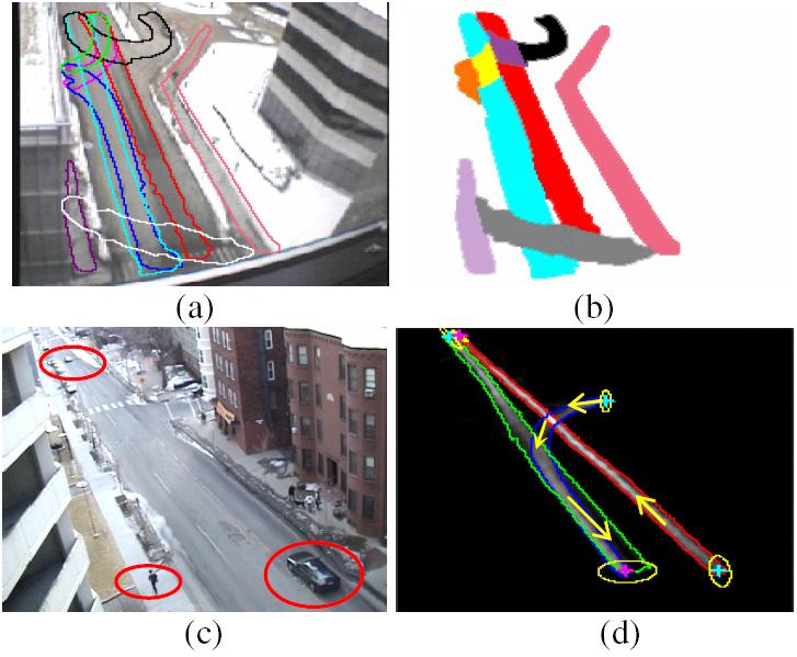
Complementary to the geometric description are the statistics of the scene. A statistical scene model provides a priori probability distributions on where, when, and what types of activities occur. It also places priors on the attributes of moving objects, such as velocity and size. Figure 1(d), shows distributions of location and direction of vehicles on three paths. A scene model may be manually input, or possibly automatically extracted from the static scene appearance. However, manual input is tedious if many scenes require labeling, and static scene appearance has large variation and ambiguity. In addition, it is difficult to handcraft the statistics of a scene, or to estimate them from static appearance alone. An example is shown in Figure 1(a)(b). From the image of scene S1, we see one road. However, the road is composed of two lanes of opposing traffic (cyan and red paths). The black path is a one-way u-turn lane. There are two entrances on the left. Vehicles from these entrances wait in the orange region in Figure 1(b) and cross the yellow region on the cyan lane in order to enter the red lane. Pedestrians cross the road via the gray region. In this work we show how this information can be automatically learned by passive observation of the scene. Our method is based on the idea that because scene structure affects the behavior of moving objects, the structure of the scene can be learned from observing the behavior of moving objects.
Figure 1. Examples of far-field scene structures
Gross positions and sizes of moving objects can be obtained from a blob tracker. A moving object traces out a trajectory of locations and sizes from entry to exit. From long-term observation we can obtain thousands of trajectories in the same scene. We propose a framework to cluster trajectories based on types of activities, and to learn scene models from the trajectory clusters. In each cluster, trajectories are from the same class of objects (vehicle or pedestrian), spatially close and have similar directions of motion. We propose two novel trajectory similarity measures insensitive to low-level tracking failures, which compare:
(I) both spatial distribution and other features along trajectories: two trajectories are similar if they are close in space and have similar feature distribution, e.g. velocity.
(II) only particular features along trajectories, and augment trajectory similarity with a comparison confidence measure. This is used to separate vehicle and pedestrian trajectories by comparing object size. Under this measure, two trajectories are similar if they have similar features, but need not be close in space. A low comparison confidence means the observed similarity may not reflect true similarity in the physical world. In far-field visual surveillance, images of objects undergo large projective distortion in different places as shown in Figure 1(c). It is difficult to compare the size of the two objects when they are far apart. The comparison confidence measure captures this uncertainty.
We propose novel clustering methods which use both similarity and confidence measures, whereas traditional clustering algorithms assume certainty in the similarities. Based on the novel trajectory similarity measures and clustering methods, we propose a framework to learn semantic scene models summarized as below. Detailed description on this work can be found in [2][3]. The method is robust to tracking errors and noise.
The scene model learning process is summarized as following.
Input: a set of trajectories obtained by the Stauffer-Grimson tracker [1] from raw video (trajectories may be fragmented because of tracking errors).
(1) Cluster trajectories into vehicles and pedestrians based on size using trajectory similarity measure II and the novel clustering methods.
(2) Detect and remove outlier trajectories which are anomalous or noisy.
(3) Further subdivide vehicle and pedestrian trajectories into different clusters based on spatial and velocity distribution using trajectory similarity I.
(4) Learn semantic scene models from trajectory clusters. In particular, sources and sinks are estimated using local density-velocity maps from each cluster, which is robust to fragmented trajectories.
(5) Real-time detection of anomalous activity using the learned semantic scene models.
See more details in [1].
We do experiments on three scnes. The results on scene S2 are shown in Figure 2. The vehicle trajectoreis and pedestrian trajectories have been first clustered into two categories using our algorithm. Then the outliers (abnormal trajectories) of vehicle trajectories and pedestrian trajectories are detected and removed, and then the remaining trajectories are clustered into different activities.
(a) |
(b) |
(c) |
(d) |
Figure 2. Clustering vehicle and pedestrian trajectories in Scene S1. (a): outlier vehicle trajectories in red; (b): six vehicle trajectory clusters (c): outlier pedestrian trajectories in red; (d): five pedestrian clusters.
In Figure 3, we show the sources and sinks of vehicles and pedestrians in Scene S3, and the boundaries of pathes discovered by our algorithm. In Figure 4 (a), outlier vehicle trajectories in S3 are marked by different colors. The green trajectory is a car backing up in the middle of the road. The car on the red trajectory first drives along the purple path in Figure 4(a), then it turns left, crosses the red path on its left side, and has opposite moving direction with the trajectories in the cyan cluster. So it is detected as an anomalous trajectory. In Figure 9 (b) we plot the log likelihood of the red trajectory in Figure 9(a) at different locations. The probability is very low when it turns left crossing the red path.
(a) Vehicles |
(b) Pedestrians |
Figure 3. Extract paths, sources and sinks of vehicles and pedestrians in Scene S3. Path boundaries are marked by different color, the source and sink centers are marked by cyan and magenta crosses. The yellow ellipses indicate the estimated extent of sources/sinks.
(a) |
(b) |
Figure 4. Detect anomalous trajectories in S3. (a): outlier trajectories; (b): transform the log-likelihood into density map. The white color indicates low probabilities (highly anomalous).
[1] X. Wang, K. Tieu and E. Grimson, “Learning Semantic Scene Models by Trajectory Analysis,” in Proceedings of European Conference on Computer Vision (ECCV) 2006. [PDF]


